Procedural City Generation in Python - Documentation
Welcome to procedural_city_generation’s documentation! In this page we will give an overview of all the things you need to know to get started with this project.
Index
- Getting it to work
- Roadmap Creation
- Polygon Extraction and Subdivision
- Creation of 3D Data
- Visualization in Blender
- Module Index
- Search Page
- Index
Getting it to work
You can get the source code at our Github Page
If you have git installed, you can clone the repository instead of downloading it as a .zip archive with:
git clone https://github.com/josauder/procedural_city_generation.git
Dependencies:
- python 2.7+
- numpy (1.8.2+)
- scipy (0.14.1+)
- matplotlib (1.4.2+)
- PyQt4 (4.8.6+)
- Blender 2.6x+
As of now, this project runs on both Python 2 and 3. All dependencies except Blender should be included in any scientific python distribution (e.g. Python(x, y) and Anaconda). To start the program with the GUI (assuming all dependencies are installed):
cd procedural_city_generation
python GUI.py
If everything worked so far, the GUI should open up and look like this:
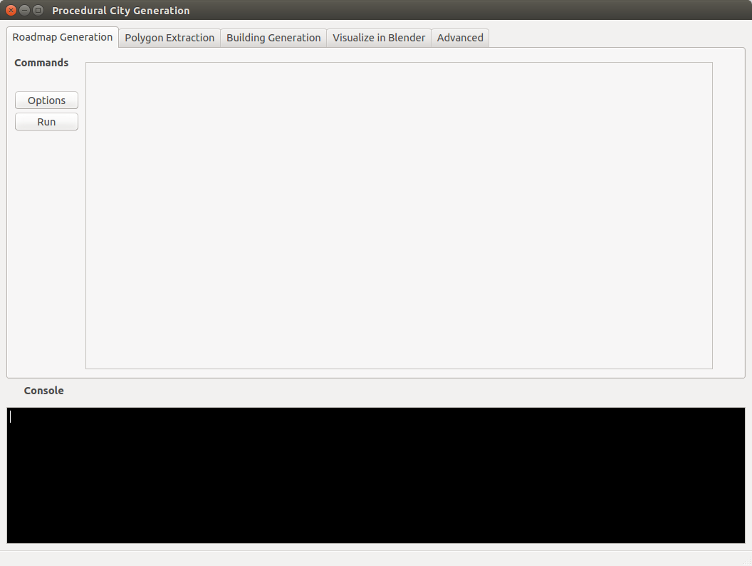
If not, then there is probably a missing dependency. To troubleshoot, try running the python file /test/Tester.py by using the following command from the procedural_city_generation directory:
python test/Tester.py
This will generate a log file in procedural_city_generation/procedural_city_generation/outputs/test.log which might contain valuable clues about why this is not working. If you can not figure it out yourself, please create an issue at our Github Page.
The last step (“Visualize in Blender”) will not work on windows machines because you can not run blender by simply typing:
blender --python "procedural_city_generation/visualization/blenderize.py"
from the command line. On windows you will have to run this script manually by opening blender, and replacing the path with the path to procedural_city_generation/procedural_city_generation directory.
About this Project
This project started as a university project at the Technische Universität Berlin. As part of the MINTGr�n Program in which students get to dedicate two semesters to enrolling in whatever courses from all STEM fields, with the goal to figure out, which of those fields they want to pursue a future in. After the semester was over, we continued working on the project though, with the goal in mind to make it usable for as many people as possible.
The entire code is open source and we are open for any feedback. If you run into any issues when using this program, please feel free to open an issue on our Github Page or even propose a fix with a pull request.
Roadmap Creation
Credits and Acknowledgements
A lot of our code regarding roadmap generation shows great similarity and in part based on the following papers:
- Martin Petrasch (TU Dresden). “Prozedurale Städtegenerierung mit Hilfe von L-Systemen”. 2008, Dresden. https://www.inf.tu-dresden.de/content/institutes/smt/cg/results/minorthesis/mpetrasch/files/Beleg_MPetrasch.pdf
- Yoav I. H. Parish (ETH Zürich), Pascal Müller (Centrap Pictures, Switzerland). “Procedural modeling of cities”. Siggraph ‘01 301-308 (2001). New York, NY, USA. https://dl.acm.org/citation.cfm?id=383292
Introduction
We refer to “road segments” as edges and the two ends of an edge as a vertex. We create roadmaps by starting with an axiom (a list of Vertices) and defining a set of rules by which new Vertices are added and connected to existing one to form Edges. Many of the terms used here become obvious when you see them in action. Let’s start by showing the most important inputs:
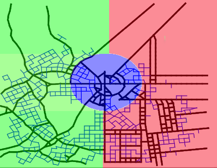
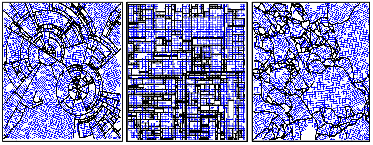
The Growth-Rule Image

This image describes which growth rule will be used in which area. Blue means that the radial rule will be used, Red means that the grid rule will be used, and Green means that the organic rule will be used. We will discuss the rules in detail later.
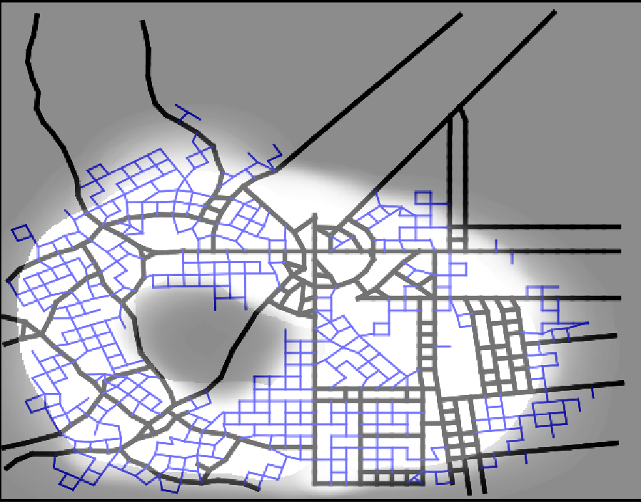
The Population-Density Image
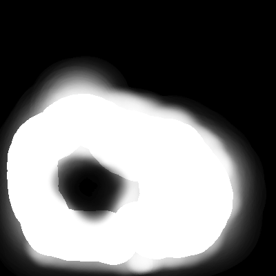
This image describes the probabilities that vertices will be connected at all. The lighter, the more probable it is, that an edge will be built.
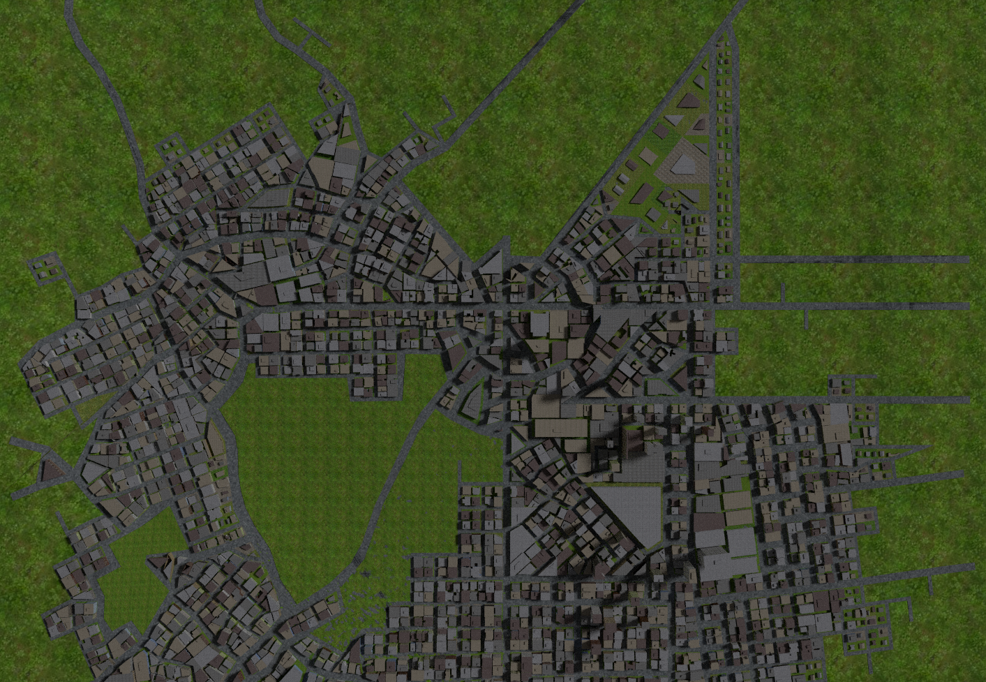
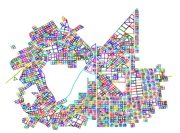
The Output
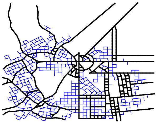
This is what the finished roadmap for a relatively small city looks like. As you see there are main roads and minor roads. The correlation between the input and the output is also very clear in this example.
Correlation between Input and Output
It should now have become clearer as to what the growth rules and the population density actually describe.
How Vertices are managed
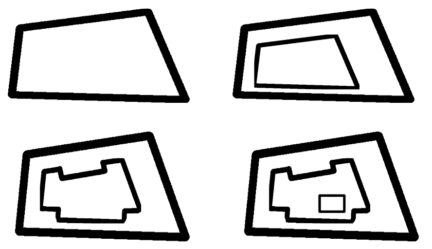
As mentioned, we start with an axiom. In the beginning, every vertex of the axiom is in the “front”, the list of vertices from which new vertices well be suggested. For every vertex, a (possibly) empty list of new suggested vertices is then created. The position of these suggested vertices depends on the growth rule. For example, if we use the grid rule, the suggested vertex for the direction “forward” is simply adding the previous edge to the vertex we are making suggestions from, and “turning” means adding this vertex rotated by either 90 or 270 degrees. All suggested vertices are then “checked” - this means we handle the following cases:
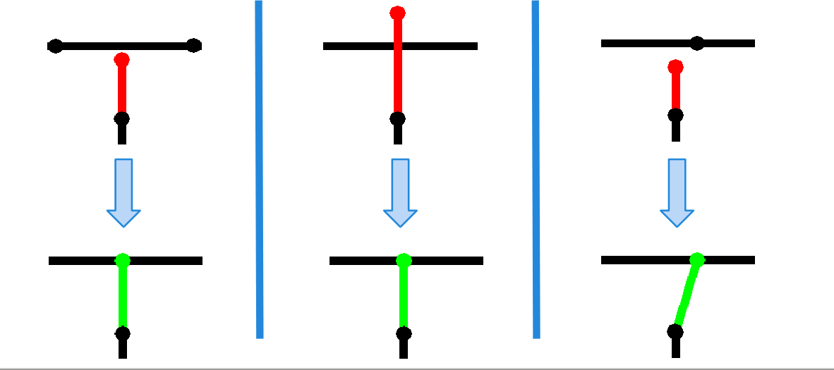
- When a new vertex is placed too close to an existing vertex, we focus on the edge to that existing vertex instead.
- When a new vertex is placed, so that the edge to that vertex stops shortly before an existing edge, we lengthen that edge to the intersection of the two edges.
- When new vertex is placed, so that the edge to that vertex intersects an existing edge, we shorten the edge to the intersection of the two edges. This also has to be checked after case 1 has been handled.
An illustation of these cases:
If none of these cases apply, the new vertex is placed and is added to the front. If there is no vertex suggested that followed the “turn” part of the growth rule, the vertex will also be added to the vertex_queue. After a vertex has spent a certain amount of iterations in the vertex_queue, it is readded to the front, under the growth rule “seed”. This growth rule starts producing vertices with the “minor_road” rule.
The Growth Rules
Below is a table describing how we suggest new vertices from a vertex by following a rule. We always need to have the previous_vector to that vertex saved.
Here you can see a demonstration of what the three main growth rules look like:
Polygon Extraction and Subdivision
We split up each of the ‘blocks’ additionally into ‘lots’. On every lot, one building can be placed. Lots that are too large will be omitted from building. The algorithm used for extracting cycles from our roadmap graph works by creating all triples of vertices which are connected, sorting these by their angle to the x-axis, making it possible to find a unique triple following each triple.
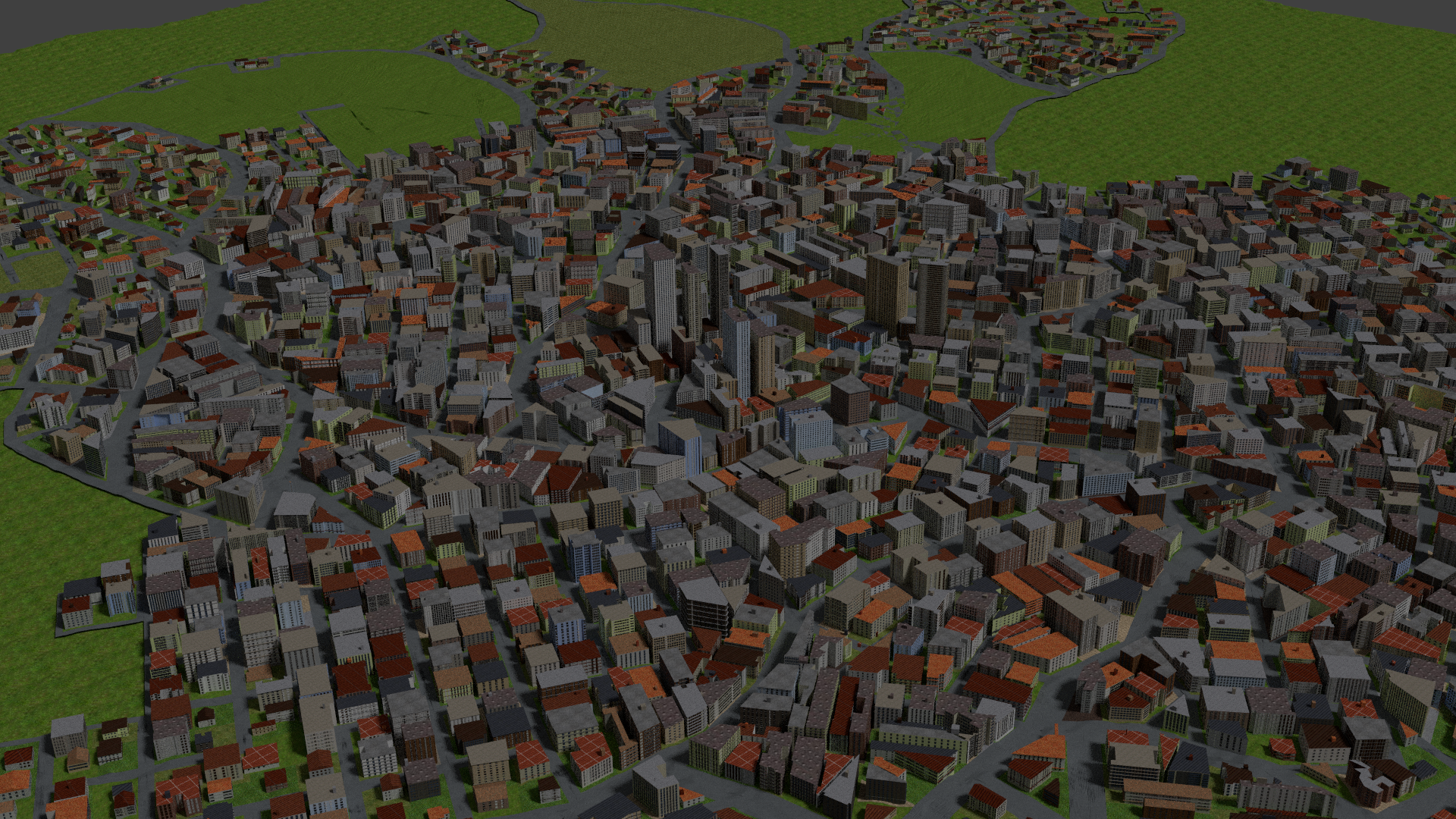
Creation of 3D Data
We create buildings by choosing various parameters according to the population density, such as the building height and Textures. We then start by scaling and or transforming the lot down, and possibly applying a series of operations on each of the walls.
Visualization in Blender
We do this by using the Blender Python API. We are not happy with performance of this API and also not happy with Blender’s memory usage (a 17x19 procedural city takes up to 6GB RAM, anything above causes a segmentation fault and a memory leak until the system is rebooted). Yet we still rely on Blender’s shrinkwrap modifier and the possibilty to use n-gons. In the future we hope to write to an .obj file, which can be opened by a plethora of 3D-Tools.